
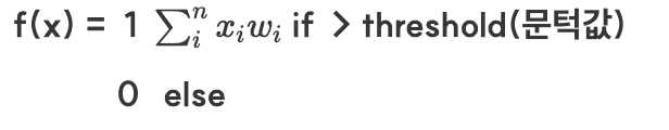
퍼셉트론을 수학적으로 다룰 때는 출력을 f(x)로 표현한다.
input*weights + bias_weights > 0.5 1? 0? -> 1 predict = 1
import numpy as np

example_input = [1,.2,.05,.1,.2]
example_weights = [.2,.12,.4,.6,.90]

input_vector = np.array(example_input)
weights = np.array(example_weights)
bias_weights = .2

activation_level = np.dot(input_vector,weights)+(bias_weights * 1)
activation_level # 0.684

# threshold
threshold = 0.5
if activation_level >= threshold:
    perceptron_output = 1
else:
    perceptron_output = 0
perceptron_output # 1
perceptron 훈련
현재는 임의의 가중치를 사용했다. 하지만 신경망의 핵심은 이런 가중치들을 신경망이 스스로 학습하고 조절하는 것이다. 퍼셉트론은 주어진 입력에 대한 추측이 맞았는지 틀렸는지에 대한 함수에 기초해서 가중치들을 증가하거나 감소함으로써 학습한다. 그런데 학습을 시작하려면 가중치들의 초깃값(initialization: 초기화)을 정해야한다. 간단한 방법으로는 난수를 이용하는 것이다. 일반적으로 정규분포 평균이 0인 난수들을 가중치로 초기화한다. 가중치들이 0이면 출력도 다 0이 되기 때문에 0에 가까운 수를 사용하여 뉴런에 너무 큰 능력을 주는 경로를 만들지 않고도 올바른 가중치를 부여할 수 있게 한다.
뉴런의 출력이 정답인지 아닌지를 토대로 가중치들을 조금씩 갱신한다. input의 갯수가 충분히 많으면 출력의 오차를 0으로 수렴하게 끔 가능하다. 각 가중치를 input값의 특징이 주는 오차에 근거해 갱신한다. 따라서 오차가 크게 나왔다면 작은 특징보다 큰 특징이 주는 오차가 크다라는 것이다.
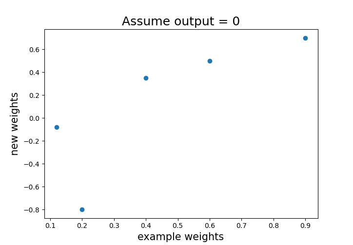
# 뉴런이 0을 출력해야한다는 가정
expected_output = 0 #예상 output
new_weights = []
for i,x in enumerate(example_input):
    new_weights.append(weights[i]+(expected_output-perceptron_output)*x)
weights = np.array(new_weights)
example_weights # 원 가중치 [0.2, 0.12, 0.4, 0.6, 0.9]
weights #  바뀐 가중치      [-0.8 , -0.08,  0.35,  0.5 ,  0.7 ]
컴퓨터 논리 학습
실전문제) 컴퓨터가 논리합(AND, OR)의 개념을 학습하게 하기, 1 AND 1 = 1 , 1 OR 0 = 1 1 AND 0 = 0 etc
# OR 학습
sample_data = [[0,0],
               [0,1],
               [1,0],
               [1,1]] # 0 : False 1 : True
expected_results = [0,
                    1,
                    1,
                    1]
activation_threshold = 0.5

from random import random #초기화
import numpy as np

weights = np.random.random(2) / 1000 # [0.00017939, 0.00062873]
weights
bias_weight = np.random.random() / 1000 #초기 가중치 난수
bias_weight # bias_weight
for idx,sample in enumerate(sample_data):
    input_vector = np.array(sample)
    activation_level = np.dot(input_vector,weights) + (bias_weights * 1)
    if activation_level > activation_threshold:
        perceptron_output = 1
    else:
        perceptron_output = 0
        print("Predicted:{}".format(perceptron_output))
        print("Expected:{}".format(expected_results[idx]))
        print()
# Predicted:0
# Expected:0
# Predicted:0
# Expected:1
# Predicted:0
# Expected:1
# Predicted:0
# Expected:1결과 1/4 4번의 시행결과 1번의 정답을 맞췄다. 반복학습으로 최적의 weight를 찾아보자
for iteration_num in range(5):
    correct_answers = 0
    for idx, sample in enumerate(sample_data):
        input_vector = np.array(sample)
        activation_level = np.dot(input_vector, weights) + (bias_weights * 1)
        if activation_level > activation_threshold:
            perceptron_output = 1
        else:
            perceptron_output = 0
        if perceptron_output == expected_results[idx]:
            correct_answers += 1
        new_weights = []
        for i, x in enumerate(sample):
            new_weights.append(weights[i]+(expected_results[idx]-perceptron_output)*x)
        bias_weight = bias_weight + ((expected_results[idx]-perceptron_output)*1)
        weights = np.array(new_weights)
        print('{} correct answers out of 4, for iteration {}'.format(correct_answers,iteration_num))

# 1 correct answers out of 4, for iteration 0
# 2 correct answers out of 4, for iteration 0
# 3 correct answers out of 4, for iteration 0
# 4 correct answers out of 4, for iteration 0
# 1 correct answers out of 4, for iteration 1
# 2 correct answers out of 4, for iteration 1
# 3 correct answers out of 4, for iteration 1
# 4 correct answers out of 4, for iteration 1
# 1 correct answers out of 4, for iteration 2
# 2 correct answers out of 4, for iteration 2
# 3 correct answers out of 4, for iteration 2
# 4 correct answers out of 4, for iteration 2
# 1 correct answers out of 4, for iteration 3
# 2 correct answers out of 4, for iteration 3
# 3 correct answers out of 4, for iteration 3
# 4 correct answers out of 4, for iteration 3
# 1 correct answers out of 4, for iteration 4
# 2 correct answers out of 4, for iteration 4
# 3 correct answers out of 4, for iteration 4
# 4 correct answers out of 4, for iteration 4결과 아주 잘 예측했다. 하지만 선형성을 띄는 예측 모델만 예측하지 비 선형성일 경우 예측 결과가 주사위 돌리는 수준이 나왔다. 이러한 문제 제기를 민스키와 패퍼트가 했다.
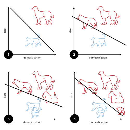

새로운 비선형 문제를 해결하기 위해 시도했지만 계산량이 너무 많았다. 논리 회로의 문제를 푸는 XOR문제 만드으로도 상당한 퍼셉트론과 상당한 분량의 역전파 계산이 필요했다. 옛날에 이러한 일을 컴퓨터에게 맡긴다는 것은 상당한 비용과 시간이 소요 되는 문제라서 인공 신경망에 대한 연구는 실용성 측면에서 빛을 보지 못했다. 하지만 2010년 초중반 루멜하트와 매클리랜드에 의해 세상으로 다시 나왔다.
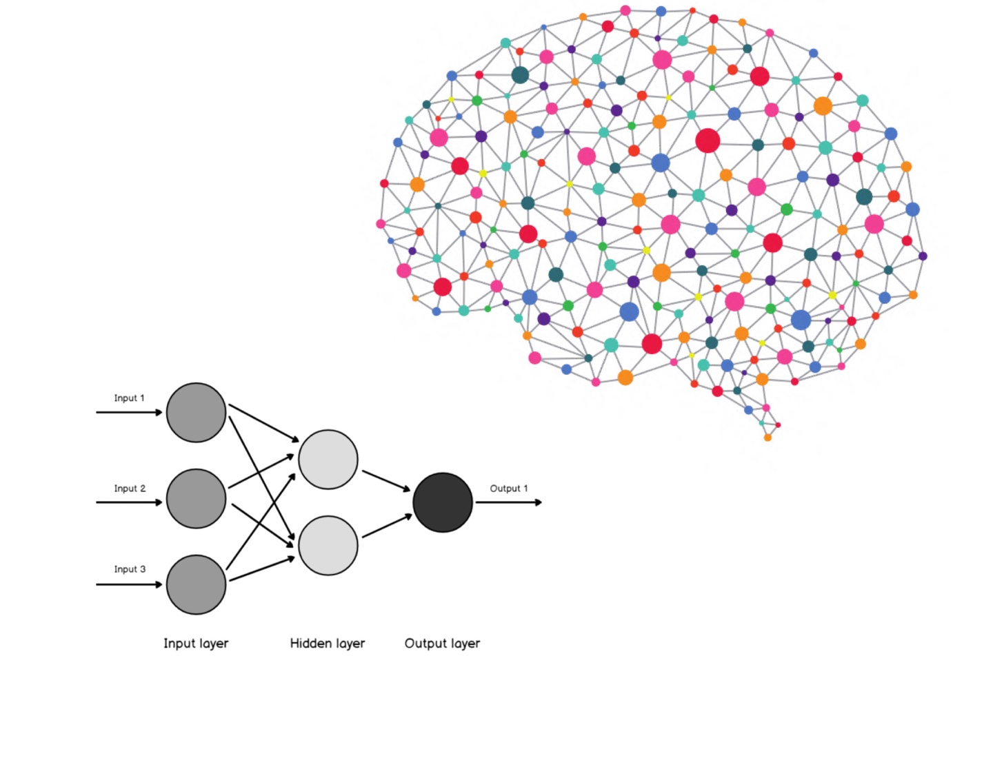
그들이 착안한 방법은 하나의 퍼셉트론으로 예측을 수행하는 대신 여러 개의 퍼셉트론을 함께 사용한 다는 것이다. 하나의 퍼셉트런에 입력을 넣고 그 퍼셉트론의 출력을 다른 퍼셉트론의 입력에 연결해서 하나의 네트워크 망을 형성한다.그 네트워크의 끝에 있는 퍼셉트론의 출력이 전체 신경망의 예측결과이다.
가중치 갱신 과정의 주요 부분을 공식화해 보면 예측 결과의 오차에 기초해서 퍼셉트론의 가중치를 갱신하는 방법을 사용한다. 그러한 오차를 측정하는 함수를 비용함수(cost function) 또는 손실함수(loss function)라 한다. 비용함수는 신경망에 입력된 '질문' 즉 입력 견본 x에 대해 신경망이 출력해야 하는 정답돠 신경망이 실제로 출력한 예측값 y의 차이를 수량화하는 함수이다. 이 손실, 비용 함수는 참값과 모형의 예측값의 차이의 절댓값을 오차 또는 비용으로 산출한다.
$err(x) = |y - f(x)|$
r"$\jmath(x) = \min\sum_{i=1}^{n}{err(x_i)}$"
이 식의 값을 최소화하는 것이 목표이다.
'👾 Deep Learning' 카테고리의 다른 글
| GAN (Generative Adversarial Networks) (0) | 2021.02.26 |
|---|---|
| 역전파 (backpropagtion) (0) | 2021.02.26 |
| [Transformer] Model 정리 (0) | 2021.02.23 |
| VAE(Variational autoencoder) 종류 (0) | 2021.02.21 |
| [Transformer] Positional Encoding (3) (0) | 2021.02.20 |